Back in September last year I wrote a series of blogs about energy uncertainty. I used a relatively simple model to estimate domestic energy prices in the future - here I'm revisiting the model and adding data published by DECC to see how the model has performed.
The graphs below show the model's performance for domestic gas prices and electricity prices. The data released by DECC in the quarterly energy statistics for the periods since I first blogged on the subject are shown in red. And as in my previous blog, the numbers shown are the price indices relative to 1987 (i.e. 1987=100) - the numbers in red show the 2Q 2013 price index and the number above it is the lower bound of the model.
The graphs below show the model's performance for domestic gas prices and electricity prices. The data released by DECC in the quarterly energy statistics for the periods since I first blogged on the subject are shown in red. And as in my previous blog, the numbers shown are the price indices relative to 1987 (i.e. 1987=100) - the numbers in red show the 2Q 2013 price index and the number above it is the lower bound of the model.
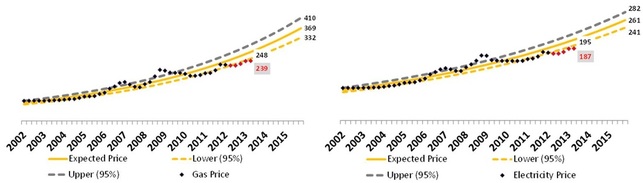
The good news (with my modeller's hat on) is that the model is working pretty well, although it is tracking the lower confidence interval rather than the expected price. However, the majority of the data points in both graphs are tracking the lower interval. This suggests that the peaks in prices in 2007 and 2009 are 'carrying more weight' than perhaps they should and that the domestic prices are mean-reverting.
So should I discount some of the outliers and re-run the model? What if there is another hike in the prices next year so that the trend might be closer to the expected price in the current model? Re-running the model without the outliers could in the latter case under estimate future energy prices - stick or twist?
Stafford Beer and Ross Ashby maintain that a model's first virtue is that it must be useful. So sticking with the model or twisting really depends on what the model's purpose is. So from my perspective, I'm going to stick because I want to see how this relatively simple modelling approach (linear regression) fares over time.
If I was using this for budgeting purposes then I would most certainly stick too as there would be money left in the energy budget (which I would then use to invest in energy reduction measures). However, if I was using this approach for project appraisal then I might consider twisting and re-running the model without the outliers and with data from 2010 onwards to compare the results. This would help to get a feel for what the risk might be to the project, particularly if you were using the expected price as an indicator of future prices and it was the savings associated with these future prices that was funding the project.
I'll revisit this model again at the end of the year to see how it has fared.

 RSS Feed
